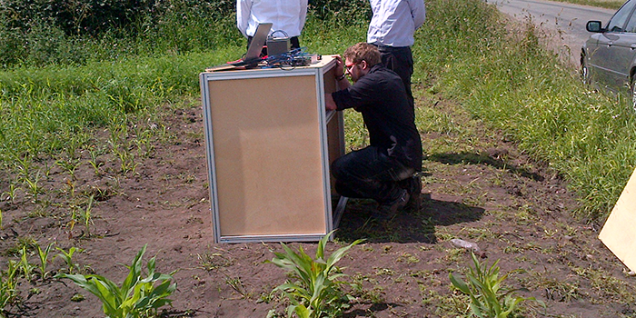
Creation of a multi-modal imaging platform for the high-precision detection of weeds in maize fields. The goal of the project was to produce a tractor-mounted device capable of classifying plant matter into “weed” or “crop” classes then detecting the meristem (growth centre) to within 2mm to allow for precision application of a treatment.

Key Technologies

C++ | OpenCV | CUDA | OpenNI | QT | Point Cloud Library | Arduino | Electronics

How Did It Work?

The platform consisted of a matched pair of computer vision cameras sporting wide-angled lenses, one for colour capture and the other specialised for near-infrared (nIR). There were 4 white/nIR illuminators on moveable attachments and structured-light RGB-D camera for coarse depth analysis.

Image Capture

• The two cameras were capable of capturing 1MP images at 200FPS, and connected over USB3.0 to a high performance workstation laptop.
• Smart image-buffering was required to handle issues with disk-write speed being slower than capture bandwidth.
• The LEDs could be strobed at high frequency to allow photometric stereo source images to be recorded.
• The strobe rate was synchronised with the camera shutter using TTL signals from the cameras’ GPIO modules.
• The configuration of lights/cameras was entirely modifiable and the software included re-calibration wizards to allow non-expert users to test different configurations.
• The system was powered from a tractor’s 12V DC supply, stepped up to 24V. This required a hardware signal filter to prevent noise in the power lines from interfering with the quality of the binary TTL signals.

2D: Real-Time Image Processing

The primary goal of the system was the detection of weeds and localisation of the meristem. For the sake of computation time, we opted for a 2D approach to solving the problem, although research was carried out on 3D data (described later). Since this had to be capable of running in real-time on a moving device at high frame-rates, it was important to achieve each step with minimal computational overhead.

We make use of colour indexes [1] as an efficient way to quickly identify plant-matter and segment it from the background. A number were considered, but Excess-Green (ExG) performed best. Essentially we take a weighted combination of the colour channels to emphasis green pixels and depress non-green.

The basic algorithm is provided below:

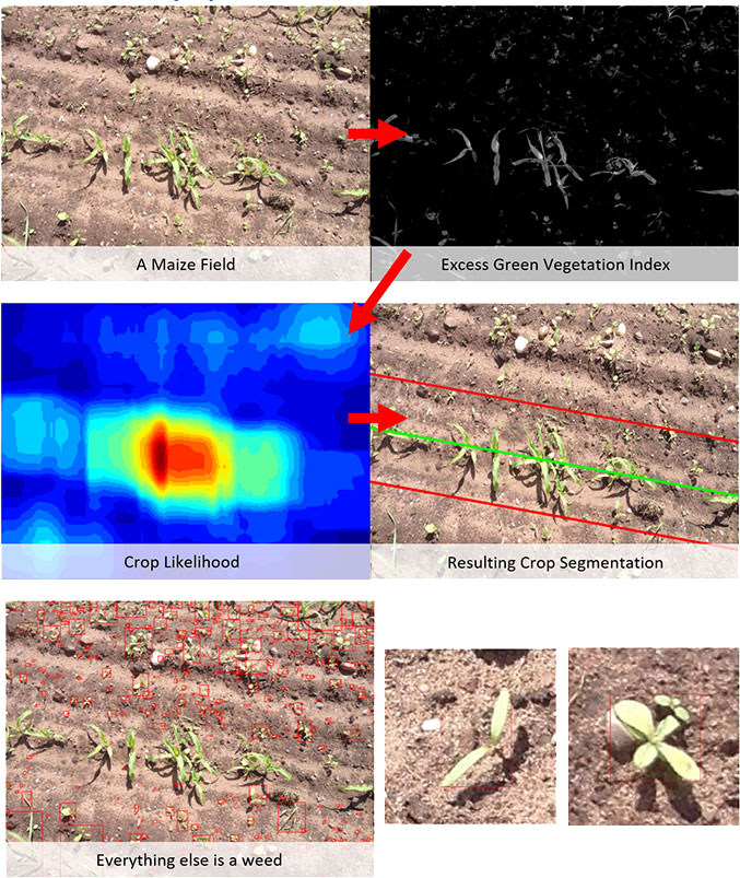
This provides us with individual weed bounding boxes, which can then be used to detect the meristem. Since grass patches are structurally different to broad-leaf weed patches, an additional classification step was added to determine the weed class.

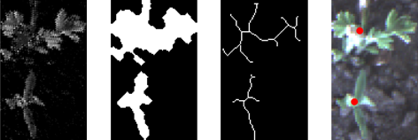
For broad-leaf patches, we use morphological techniques to skeletonise the patch blob, then examine branch points in the skeleton to estimate the meristem location. The system was robust to segmentation errors where multiple plants might get merged into the same box at global scale:

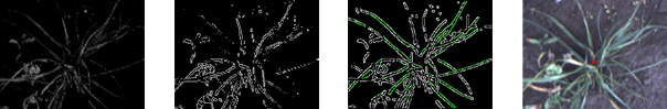
For grassy patches, we observed that there were typically strong lines directed from the extremity of the plant to the growth point. We could then use traditional image processing techniques such as Canny edge detection and Hough line detection to quickly and efficiently estimate the growth centre:

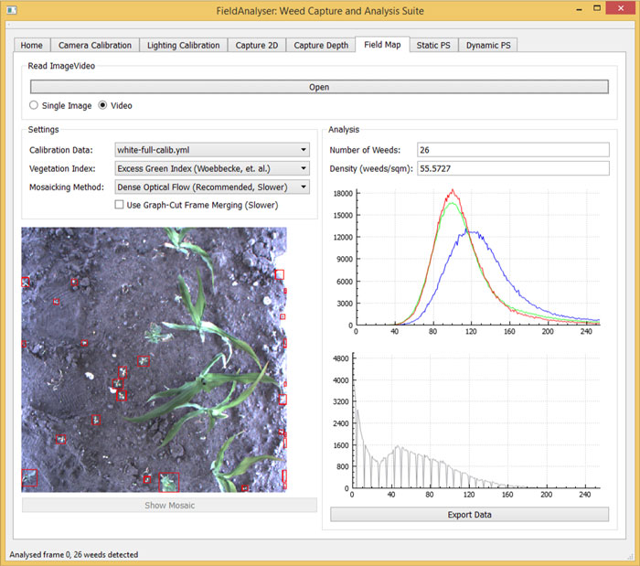
The algorithms developed for this project were incorporated into a software suite, an example of which (running on real field data) is shown below:

3D Analysis

By strobing the lights in time with the camera shutter, the system was capable of 4-light and 2-light photometric stereo, reconstruction, both in nIR and colour. Since the frame-rate of the camera is 200Hz, we achieve either a capture rate of 100Hz or 50Hz, depending on the number of source images captured.

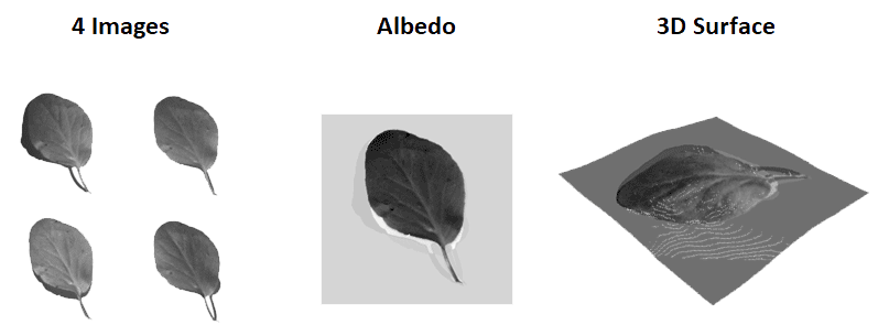
The four-light technique for surface calculation runs slowly, since we must solve a series of equations at each pixel (for more details, checkout my related blog post on Photometric Stereo). If we wish to run in real-time, we can use the two-light, optimised photometric stereo method from [2].

Rather than a full surface normal field, we instead obtain the surface gradient in the axis parallel with the two light sources (referred to as 2.5D):

By dividing by , we obtain the gradient:

This work focused primarily on the capture of various image modalities, so analysis of the resulting 2.5D and 3D imagery was not part of the project; however intuition suggests that using metrics such as Koenderink’s Shape Index [] and the HK Segmentation [] would provide good starting points for image analysis. It would also be reasonable to apply machine learning approaches to the surface normals or gradients to provide a data sample which is more robust to aesthetic variations and more focused on plant structure.

It should also be noted that Photometric Stereo provides only pixel-wise surface orientation. While we can reconstruct an estimate of 3D shape by integrating over the normal field, this is rarely correct in the depth-axis. By combining the high-resolution surfaces from PS with the low quality, but metrically correct depth maps, we could potentially produce metric-rectified high resolution 3D models.

[1] G. E. Meyer and J. a. C. Neto. Verification of color vegetation indices for automated crop imaging applications. Computers and Electronics in Agriculture, 63(2):282–293, Oct. 2008. ISSN 01681699.

[2] J. Sun, M. L. Smith, A. Farooq, and L. N. Smith. Counter camouflage through the removal of reflectance. ICMV 2010, Dec. 2010. URL http: //eprints.uwe.ac.uk/11992/.

[3] J. Koenderink and A. van Doorn, “Surface shape and curvature scales,” IVC, vol. 10, pp. 557-565, 1992.

[4] P.J. Besl. Surfaces in range image understanding. Springer, 1988